I learned a lot about financial crises from Gary Gorton's work in the area. His views on what went wrong during the recent crisis and what might be done to prevent similar events are views that should be taken seriously. Seriously, that is, but not uncritically. And this is where George Selgin provides a useful service: see Misunderstanding Financial History.
Wednesday, 31 July 2013

Saturday, 29 June 2013
Sadowski on Bullard (Guest Post)
About a year ago, Jim Bullard criticized the argument that that the Fed was missing on both sides of its dual mandate. Mark Sadowski (who should have his own blog, I think) has asked me to post his reply. I am most happy to do so.
=======================================
=======================================
This is written in response to a question David Andolfatto posed in September in a blog post entitled “Is the Fed missing on both sides of its dual mandate?”
David concluded that post with the following statement:
“Bullard suggests that a non-monotonic transition path for inflation is unlikely to be part of any optimal path in a NK [New Keynesian] type model. The optimal path for inflation is unlikely to be part of any optimal path in a NK type model. The optimal transition dynamics are typically monotonic—think of the optimal transition path as a movement back up the PC [Phillips Curve] in the diagram above. If this is true, then the optimal transition path necessarily has the Fed missing on both sides of its dual mandate.
Of course, conventional NK models frequently abstract from a lot of considerations that many people feel are important for understanding the recent recession and sluggish recovery. The optimal monetary policy may indeed dictate "inflation overshooting" in a different class of models. Please feel free to put forth your favorite candidate. Tell me why you think Bullard is wrong.”
James Bullard, President of the St. Louis Fed, had just written an opinion piece for the Financial Times where he stated:
“To argue against monotonic convergence now would imply that when unemployment is above the natural rate, monetary policy should aim for inflation above the Fed’s 2 per cent target. On the face of it, this does not make sense: the US has experienced periods when both inflation and unemployment have been above desirable levels. In the 1970s this phenomenon was labeled stagflation. Monetary policy has been regarded as poor during that period.”
At the time Scott Sumner mockingly responded:
“To argue for monotonic convergence now would imply that when unemployment is above the natural rate, monetary policy should aim for inflation below the Fed’s 2 per cent target. On the face of it, this does not make sense: the US has experienced periods when both inflation and employment have been below desirable levels. In the 1930s this phenomenon was labeled “The Great Depression.” Monetary policy has been regarded as poor during that period.”
Sumner is of course talking about the contractionary portion of the U.S. Great Depression. The subsequent 1933-37 recovery, during which real GDP grew at an average rate of 9.5%, is an excellent example of “oscillatory convergence” with unemployment high and falling and inflation higher than normal. And yes, monetary policy is generally regarded as excellent during that period.
Andolfatto’s, Bullard’s, and Sumner’s comments raise a great many questions. For example, what is the relationship between unemployment and inflation? How has this relationship changed over time, and why? How has this relationship been modeled over time? How should this relationship affect the conduct of monetary policy? For the moment, at least, I want to stay focused on Bullard’s remarks.
As evidence Bullard cited a paper by Frank Smets and Raf Wouters, “Shocks and Frictions in US Business Cycles – A Bayesian DSGE Approach” (American Economic Review, Vol. 97, No. 3, June 2007, pp. 566-606). In an essay published about a month later, “Monetary Policy and the Expected Adjustment Path of Key Variables” (Federal Reserve Bank of St. Louis Economic Synopses, 2012, No. 30), Bullard clarified his Financial Times comments:
“Let’s consider the medium-sized macroeconomic framework of Smets and Wouters (2007). This is an important benchmark model; and, while we could argue about the details, I think it will serve to make my point. In the Smets and Wouters dynamic stochastic general equilibrium (DSGE) model there are many shocks, and there is a monetary policymaker that follows a Taylor-type monetary policy rule not unlike ones used in actual policy discussions. The authors estimate their model using postwar U.S. data, and they also report results for subsamples including the post-1984 data. Importantly, what the authors are estimating is a general equilibrium for the economy, which includes monetary policy.
How does the economy adjust in the Smets and Wouters model? The chart is Figure 2 from their paper.
The authors plot the reaction of key macroeconomic variables to three types of shocks in their model that might be thought of as demand shocks. Variables are reported as deviations from a steady-state value, so that zero represents a return to normal. The variables include inflation and a labor market variable—hours worked. Time is measured in quarters. The shock is a positive one—output and hours go up in response—but the story is merely transposed for a negative shock (i.e., flip the figures upside down).
The reaction of all variables is essentially monotonic beyond the hump in these graphs, at least through year four. (That is, the adjustment does not show much of a tendency to oscillate about the long-run value.) For all three types of demand shocks, the Fed would be “missing on both sides of the dual mandate” almost all of the time as the economy recovers from the shock. If the shock were negative, hours would be too low (unemployment too high), and inflation would be too low every quarter for many years. Yet the monetary policy embedded in this general equilibrium is a Taylor-type policy rule that has often been argued to closely approximate the optimal monetary policy in frameworks such as this one. 2 It is in this sense that I do not think merely observing where inflation and unemployment are relative to targets or long-run levels at a point in time is telling us very much about whether the monetary policy in use is the appropriate one or not.”
Footnote 2 reads:
“One can investigate optimal-control monetary policy assuming credible commitment in this model, taking the non-policy parameters as estimated by Smets and Wouters. This type of monetary policy changes these impulse response functions but still leaves goal variables “missing on both sides of the mandate” in many situations. I thank Robert Tetlow for investigating this issue in response to an earlier draft.”
The monetary policy reaction function that is built into the Smets and Wouters (2007) model is the original rule John Taylor proposed in 1993 ("Discretion versus Policy Rules in Practice", Carnegie-Rochester Conference Series on Public Policy, Vol. 39, December 1993, pp. 195-214), namely a Taylor Rule that places equal weights on the inflation gap and the output gap. In 1999 Taylor discussed an alternative version of this rule that placed double the weight on the output gap than on the inflation gap, (“A Historical Analysis of Monetary Policy Rules”, Monetary Policy Rules, Chicago: University of Chicago Press, pp. 319-341). This is a point to which we shall return later. Thus the response of the economy to the demand shocks illustrated in Figure 2 is conditional on the Taylor Rule embedded in the model.
At this point it might be worth mentioning that one of the acknowledged shortcomings of medium-scale New Keynesian DSGE models is that typically there is no reference to unemployment. Bullard infers the impact of a demand shock on unemployment from its effect on hours worked. In particular, the Phillips Curve in the Smets-Wouters model is a hybrid New Keynesian type in which inflation depends on past inflation, expected future inflation, current price mark-up and a price mark-up disturbance. Apparently the only reference in the model to the output gap occurs in the model’s monetary policy reaction function (i.e. the Taylor Rule).
Bullard’s footnote on optimal control monetary policy is especially relevant in this context. What is “optimal control” monetary policy? Federal Reserve Vice Chair Janet Yellen spoke about optimal control techniques in speeches in April, June and November of last year. Here is how she introduced them in April:
“One approach I find helpful in judging an appropriate path for policy is based on optimal control techniques. Optimal control can be used, under certain assumptions, to obtain a prescription for the path of monetary policy conditional on a baseline forecast of economic conditions. Optimal control typically involves the selection of a particular model to represent the dynamics of the economy as well as the specification of a "loss function" that represents the social costs of deviations of inflation from the Committee's longer-run goal and of deviations of unemployment from its longer-run normal rate. In effect, this approach assumes that the policymaker has perfect foresight about the evolution of the economy and that the private sector can fully anticipate the future path of monetary policy; that is, the central bank's plans are completely transparent and credible to the public."
In that speech Yellen describes how projections generated by FRB/US, the Federal Reserve’s primary forecasting model, were adjusted to replicate the baseline outlook constructed using the distribution of FOMC participants' projections for unemployment, inflation, and the federal funds rate that were published in January of that year. A search procedure was used to solve for the path of the federal funds rate that minimized the value of a loss function. The loss function was equal to the cumulative sum from 2012:Q2 through 2025:Q4 of three factors: 1) the discounted squared deviation of the unemployment rate from 5-1/2 percent, 2) the squared deviation of overall PCE inflation from 2 percent, and 3) the squared quarterly change in the federal funds rate. She termed this path the “optimal control” path.
Yellen also used the FRB/US model to construct the federal funds rate path called for by the 1993 and 1999 versions of the Taylor Rule conditioned on the same illustrative baseline outlook used to generate the optimal control path. These paths, as well as the optimal control, and the various resulting paths for unemployment and inflation are depicted in Figure 8 of her speech:
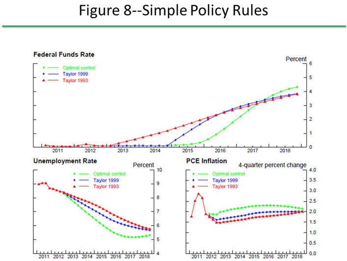
The 1993 Taylor Rule calls for the federal funds rate to begin rising in 2013Q2. The 1999 Taylor Rule calls for the federal funds rate to begin rising in 2015Q1. Optimal control calls for the federal funds rate to begin rising in 2015Q4. More importantly, note that whereas the paths for unemployment and inflation under the Taylor Rules converge monotonically, under optimal control they display oscillatory convergence, with both unemployment and inflation “overshooting” before converging to their long run values.
Now, it’s true these results were generated with FRB/US and not the Smets-Wouters model. FRB/US is a somewhat older (1997), large-scale simultaneous equation macroeconometric model. But because expectations of future economic conditions are explicit in many of its equations, and adjustment of nonfinancial variables is delayed by frictions, it too is often described as New Keynesian. The dynamic adjustment of its aggregate price equation means that, like the Smets-Wouters model, inflation is dependent on past inflation, expected future inflation and the current price markup, as well as number of additional variables such as the unemployment rate, energy prices, etc. And the general effect of monetary policy shocks on output, inflation and interest rates is quite similar to the Smets-Wouters model.
Thus I expect were one to investigate optimal control monetary policy assuming credible commitment using the Smets-Wouters model, as Bullard mentions the possibility of in his footnote, one would probably find results similar to those generated with the FRB/US model assuming it were subject to the same loss function. To be more explicit, under the same assumptions, an optimal control path generated by the Smets-Wouters model would very likely exhibit the same oscillatory convergence pattern of unemployment and inflation as demonstrated with the FRB/US model.
Thus it seems to me that the primary issue here is not what type of model should be used, but what the goals of monetary policy should be. Should monetary policy be guided by simple rules, such as the Taylor Rules, because in the past, and under potentially very different conditions, they were considered optimal? Or should monetary policy be more explicitly guided by the mandates to which it is legally subject? Or, indeed, should monetary policy be guided by something else entirely?
Mark Sadowski
Mark Sadowski
Wednesday, 24 April 2013
Why gold and bitcoin make lousy money

Is it important for a monetary instrument to hold its value over long periods of time? I used to think so. But now I'm not so sure. While I do not necessarily like the idea of inflation eating away at the value of fiat money, I don't think that a low and stable inflation rate is such a big deal. Money is not meant to be a long-term store of value, after all. Once you receive your wages, you are free to purchase gold, bitcoin, or any other asset you wish. (Inflation does hurt those on fixed nominal payments, but the remedy for that is simply to index those payments to inflation. No big deal.)
I find it interesting to compare the huge price movements in gold and Bitcoin recently, especially since the physical properties of the two objects are so different. That is, gold is a solid metal, while Bitcoin is just an abstract accounting unit (like fiat money).
But despite these physical differences, the two objects do share two important characteristics:
[1] They are (or are perceived to be) in relatively fixed supply; and
[2] The demand for these objects can fluctuate violently.
[2] The demand for these objects can fluctuate violently.
The implication of [1] and [2] is that the purchasing power (or price) of these objects can fluctuate violently and at high frequency. Given [2], the property [1], which is the property that gold standard advocates like to emphasize, results in price-level instability. In principle, these wild fluctuations in purchasing power can be mitigated by having an "elastic" money supply, managed by some (private or public) monetary institution. This latter belief is what underlies the establishment of a central bank managing a fiat money system (though there are other ways to achieve the same result).
The following graph depicts the rate of return on US money over the past century (the rate of return is actually the inverse of the inflation rate). The US was on and off the gold standard many times in its history. Early on in this sample, the gold standard was abandoned during times of war and re-instituted afterward. While inflation averaged around zero in the long-run, it was very volatile early in the sample. The U.S. last went off the gold standard in 1971. Later on in the sample, we see the great "peacetime inflation," followed by a period of low and stable inflation.

Gold standard advocates are quick to point out the benefits of long-term price-level stability. The volatile nature of inflation early on in the sample is attributed to governments abandoning the gold standard. If only they would have kept the gold standard in place...
Of course, that is the whole point. A gold standard is not a guarantee of anything: it is a promise made "out of thin air" by a government to fix the value of its paper money to a specific quantity of gold. It is possible to create inflation under a gold standard simply by redefining the meaning of a "dollar." For example, in 1933, FDR redefined a dollar to be 1/35th of an ounce of gold (down from the previous 1/20th of an ounce). This simple act devalued the purchasing power of "gold backed money" by almost 60%.
If the existence of a gold reserve does not prevent a government from reneging on its promises, then why bother with a gold standard at all? The key issue for any monetary system is credibility of the agencies responsible for managing the economy's money supply in a socially responsible manner. A popular design in many countries is a politically independent central bank, mandated to achieve some measure of price-level stability. And whatever faults one might ascribe to the U.S. Federal Reserve Bank, as the data above shows, since the early 1980s, the Fed has at least managed to keep inflation relatively low and relatively stable.
Monday, 15 April 2013
This is not rocket science

He seems to think that some people in the profession are confused about things like the natural rate of interest and its relation to the market rate. What's ailing the economy is so painfully obvious. Why are these dopes trying to make things harder than they are? This is not rocket science after all.
Well, I freely admit to being a bit confused. Let me explain why.
First, the "natural rate of interest" is a term that seems to mean different things to different people. According to DeLong, the natural rate of interest is the (real) interest rate consistent with "full employment." Well, that's all fine and good, except that he does not define what he means by "full employment." (I certainly hope he does not define it as the level of employment consistent with the natural rate of interest!)
In my view, the natural rate of interest and the full employment level of employment are theoretical objects. They may or may not exist in reality. Economists use these terms to help them interpret the world. Nobody knows for sure just by looking at the data where the economy sits in relation to the natural rate of interest or full employment (however these terms are defined theoretically).
One might of course try to estimate their values by sample averages in the data. But this approach is not without problems. The employment-population ratio in the U.S. shows secular variation. Moreover, it varies across different demographic groups. Take a look at this, for example. While there are more sophisticated ways of estimating these things, the whole exercise is predicated on the assumption that these objects actually exist. (They most certainly do, if only in the minds of some economists).
In any case, with that little bit out of the way, I'd like to see whether I can make sense of the various claims that DeLong makes in his column.
1. The current natural interest rate is much lower than it is normally--the natural rate is too low--and that is a problem.
One way to understand this statement is with the classic "loanable funds" market diagram. There is a supply for loanable funds S(r,Y), increasing in the real interest rate r, and increasing in the level of real income Y. The the demand for loanable funds, or investment demand, I(r) is a decreasing function of r. Let Y* denote the full-employment level of GDP. Then, in a closed economy, the natural rate of interest r* satisfies S(r*,Y*) = I(r*).
Now, imagine that investment demand collapses for some reason. Moreover, assume that the zero lower bound (ZLB) is not binding. What happens to the full-employment level of Y? I am not sure what DeLong is assuming here. I think he assumes that it remains unchanged at Y*, but that actual Y may move along some "short run" (sticky price) AS curve. So, are we currently in the short-run or long-run? He does not say. I say that after four years, the sticky price frictions are probably no longer relevant, especially since U.S. CPI is close to its long-run trend. If this is the case, then he must be assuming that Y* is currently at its pre-crisis level (or would be, if the ZLB was not a problem).
But what is the problem here? If the interest rate is free to move, then the economy achieves full employment and GDP remains at "potential" Y*. (This, despite the collapse in investment, which lowers the future capital stock, future real GDP, etc.? How can Y* remain unchanged years after lower-than-normal investment?) I am led to infer from this discussion that he views the real problem as stemming from the ZLB, which he tackles in his next statement.
2. The current market interest rate is higher than the natural rate--the market rate is too high--and that is a problem.
Alright, suppose that r0 cannot be attained because of the ZLB on nominal interest rates (despite the fact that yields on longer maturities are not at the ZLB, but anyway, ignore this too.) Then the market interest rate r1 is too high; i.e. r1 > r0. If this situation persists, then according to this simple model, the level of output must decline to some Q satisfying S(r1,Q) = I(r1); where Q < Y*. This is also a problem; see also Krugman.
If this latter problem is indeed the problem, then there are simple fixes. First, the Fed could raise its inflation target. Inflation serves as a tax on saving because it lowers the real rate of interest (given the ZLB). At the same time, it stimulates spending. The fiscal authority could achieve the same result by just taxing saving directly. I wonder, however, how many people really believe this to be *the* problem.
*The* problem seems more related to whatever caused the collapse in investment demand in the first place. I'm sure that most economists, including DeLong, would agree with this. But the key question, in my view, is precisely what factors (institutional arrangements and exogenous shocks) caused the collapse and whether the desired policy response should be made contingent on specific causes. My experience in working with economic models is that the optimal policy response generally depends a great deal what one assumes about the underlying shock. I believe that this lesson likely holds for real economies too and I wish that economists would spend more time talking about this.
3. Increasing G--printing more Treasury bonds, selling them, and buying goods and services--(a) increases the supply of safe assets, (b) lowers the proper value of safe assets via supply and demand, thus (c ) raises the "natural" rate of interest, and (d) could fix our problems if the policy raises the natural rate of interest so much that it is no longer lower than the market rate of interest.
Listen folks, I am not against increasing government spending (see for example, here). But we have to be clear about what economists mean by "increasing G." What they mean is an increase in spending in any form. This is the proverbial "digging up holes and filling them up again" prescription. Or Krugman's famous "let's build a bunch of stuff and export it to Mars" prescription. Of course, they do not mean that this is the way resources should be used. The statement is simply that even if the resources were to be used in a wasteful manner, it would work. Well, forgive me for not being so comfortable with that proposition.
Now, suppose we instead take Steve Williamson's view (more correctly, my interpretation of his view) that the collapse in investment spending is related to the evaporation of private label liquidity products (like the MBS products that used to circulate in the repo market). In fact, Steve has an interesting paper where he lays out the details of a specific model here: Liquidity, Monetary Policy, and the Financial Crisis. Brad may want to read this himself, once he works his way through Wicksell.
Unfortunately, there is no simple way to summarize Williamson's model in a short blog post. As in reality, what happens depends on a specific set of circumstances. In one case he considers, the shock that afflicts the banking sector drives up the demand for relatively safe securities, which drives the real interest rate down. Hence, the statement that "the interest rate is too low" (relative to the rate that would prevail if the economy worked perfectly). There is no talk of "natural" rate of interest or "full employment" in Willamson's paper. In Descartes-like fashion, we could say that Willamson had no use for that language.
In his model (as in reality), U.S. Treasuries are substitutes for the now missing private collateral objects. In his "scarce interest-bearing asset" case, a one time open market operation by the Fed (purchase of UST) has a perverse effect: it diminishes the supply of good collateral and therefore raises its price; i.e., it lowers the real interest rate--but in a way that is bad for the economy because it further depresses investment (that is, the lower interest rate is a reflection of a downward shift in the investment demand schedule.) Williamson calls this the "illiquidity effect."
[Note: I am not arguing that this is in fact what is happening. It may or may not constitute one of many forces that are currently in operation. It is a property that emerges from a standard economic model with realistic frictions. It is standard practice to use theory to help guide us what to look for in the data. For example, it was theory that motivated modern day NIPA design, not the other way around!]
The policy prescription in Williamson's model is for the Treasury to expand its supply of debt, both to meet the hightened demand and to cover for the shortfall in (private) supply. What is the Treasury to do with its proceeds? In principle, the Treasury could buy up private securities (this is like a banking operation--an open market operation, but with Treasuries instead of money). Or taxes could be cut. Or, yes, an increase in G too (but whether and how much to do this should be based on standard cost-benefit calculations.)
Unlike the "this is not rocket science model" that DeLong likes to work with, there are many interesting cases that emerge in the Williamson model. Macroeconomists should go read it. His paper is by no means the last word on the subject. Indeed, it may turn out one day to be all wrong. But that is the nature of research. There are still a lot of things we do not understand about the way the macroeconomy works. Well, for those of us who remain confused, in any case.
Thursday, 11 April 2013
Monetary policy in a liquidity trap
Krugman has an interesting article today, Monetary Policy in a Liquidity Trap. I (sort of) agree with much of it. But I believe that a few comments are in order.
Consider this statement:
First, the quoted passage above suggests that a liquidity trap is the byproduct of "insufficient private demand," with the implication, of course, that more "public demand" is needed to rectify the situation. This may or may not be true. Regardless, the statement is [1], [2], and [3] above. Beware of economists making bald assertions.
Second, the statement is wrong in suggesting that our current liquidity trap is associated with zero nominal interest rates. Liquidity trap phenomena are much more general than this. And if you really want to further your understanding on this matter, please go read this piece by Steve Williamson: Liquidity Traps, Money, Inflation, and Bond Yields. As Steve says: this is not your grandma's liquidity trap.
In grandma's liquidity trap, the real interest rate is too high because of the zero lower bound. Steve argues that in our current liquidity trap, the real interest rate is too low, reflecting the huge world appetite for relatively safe assets like U.S. treasuries.
If this latter view is correct, then "corrective" measures like expanding G or increasing the inflation target are not addressing the fundamental economic problem: low real interest rates as the byproduct of real economic/political/financial factors.
Given these "real" problems, Steve's view is that the Fed is largely irrelevant. But he does assign hope to the Treasury: increase the supply of its securities to meet the world demand for them. I've been making similar arguments for some time now; for example, here.
Apart from all this, it will be interesting to see how the experiment in Japan plays out. Most of the massive purchases announced by the BOJ are for JGBs -- I'm really skeptical what sort of effect this should have (since the operation constitutes swaps of two assets that are close to perfect substitutes--although some purchases will take the form of higher risk assets--see Noah Smith on this). But what I think really does not matter--it is what market participants think--and the program does appear to be having some effect in financial markets.
Thank you, Japan, for this interesting experiment. Domo arigato, gozaimasu!
Consider this statement:
So, at this point America and Japan (and core Europe) are all in liquidity traps: private demand is so weak that even at a zero short-term interest rate spending falls far short of what would be needed for full employment. And interest rates can’t go below zero (except trivially for very short periods), because investors always have the option of simply holding cash.This statement is, in varying degrees: [1] interpretative, [2] assertive, [3] misleading, and [4] wrong.
First, the quoted passage above suggests that a liquidity trap is the byproduct of "insufficient private demand," with the implication, of course, that more "public demand" is needed to rectify the situation. This may or may not be true. Regardless, the statement is [1], [2], and [3] above. Beware of economists making bald assertions.
Second, the statement is wrong in suggesting that our current liquidity trap is associated with zero nominal interest rates. Liquidity trap phenomena are much more general than this. And if you really want to further your understanding on this matter, please go read this piece by Steve Williamson: Liquidity Traps, Money, Inflation, and Bond Yields. As Steve says: this is not your grandma's liquidity trap.
In grandma's liquidity trap, the real interest rate is too high because of the zero lower bound. Steve argues that in our current liquidity trap, the real interest rate is too low, reflecting the huge world appetite for relatively safe assets like U.S. treasuries.
If this latter view is correct, then "corrective" measures like expanding G or increasing the inflation target are not addressing the fundamental economic problem: low real interest rates as the byproduct of real economic/political/financial factors.
Given these "real" problems, Steve's view is that the Fed is largely irrelevant. But he does assign hope to the Treasury: increase the supply of its securities to meet the world demand for them. I've been making similar arguments for some time now; for example, here.
Apart from all this, it will be interesting to see how the experiment in Japan plays out. Most of the massive purchases announced by the BOJ are for JGBs -- I'm really skeptical what sort of effect this should have (since the operation constitutes swaps of two assets that are close to perfect substitutes--although some purchases will take the form of higher risk assets--see Noah Smith on this). But what I think really does not matter--it is what market participants think--and the program does appear to be having some effect in financial markets.
Thank you, Japan, for this interesting experiment. Domo arigato, gozaimasu!
Wednesday, 10 April 2013
Poor Germany
Well, here's an eyebrow raiser: Germans Among Poorest in Europe: ECB Study.
The paper is available here: The Eurosystem Household Finance and Consumption Survey. The cross country comparison of net wealth can be found in Table 4.1 on page 76.
Median net wealth in Germany for 2010 was 51K eur. Compare this to median wealth in Greece (101K), Italy (173K) and Spain (182K).
This just doesn't sound right to me, but I haven't gone through the report in detail. Evidently, the differences are driven primarily by real estate wealth. Thankfully (?), Germany escaped the housing price "bubble" that afflicted many European countries; see figure below.

Moreover, as I noted here, the German growth experience over the past 20 years has been nothing to write home about.
Germany: low growth, no asset price bubbles, low wealth, but...stable. Das ist gut?
April 16, 2013: Update here from VOX, who emphasize that the wealth distribution in Germany distorts the picture presented here.
The paper is available here: The Eurosystem Household Finance and Consumption Survey. The cross country comparison of net wealth can be found in Table 4.1 on page 76.
Median net wealth in Germany for 2010 was 51K eur. Compare this to median wealth in Greece (101K), Italy (173K) and Spain (182K).
This just doesn't sound right to me, but I haven't gone through the report in detail. Evidently, the differences are driven primarily by real estate wealth. Thankfully (?), Germany escaped the housing price "bubble" that afflicted many European countries; see figure below.

Moreover, as I noted here, the German growth experience over the past 20 years has been nothing to write home about.
Germany: low growth, no asset price bubbles, low wealth, but...stable. Das ist gut?
April 16, 2013: Update here from VOX, who emphasize that the wealth distribution in Germany distorts the picture presented here.
Tuesday, 19 March 2013
Krugman on Taylor
I had five minutes to kill so I read this: Cogan, Taylor and the Confidence Fairy, by Paul Krugman.
Let's see, what do we have here? Ah, yes...I see Krugman accusing Taylor of being dishonest. Paulo, Paulo...tsk tsk.
To be more specific, Krugman accuses Cogan and Taylor of dishonesty concerning the current state of macroeconomic research. The claim they made was that expectations did not play and explicit role in "old style" Keynesian models. Of course, Keynes and most of the other great economists of the 19th and early 20th centuries assigned a critical role to expectations. But if by "old style" Keynesian models we mean Hicks' IS-LM representation of (a part of) Keynes' theory, then Cogan and Taylor are largely correct. For example, do you see expectations entering explicitly anywhere in this exposition?
By the way, I find it a bit of a hoot that it is Krugman complaining that others in the field are not keeping abreast with the literature. Steve Williamson has addressed this on more than one occasion; see here, for example. But anyway, this is getting rather tiresome.
In fact, it appears that Krugman did not even read the Cogan and Taylor paper. Fortunately, Noah Smith helps lift the lazyman's load: John Taylor's Austerity Model. (Oh gosh, it appears that their results have nothing to do with the "confidence fairy." Oh well, "confidence fairy" looks so good in the title of a NY Times Op-Ed piece.) Noah summarizes his assessment of their work as follows:
Unfortunately, Noah stumbles a bit on the partisan divide with this concluding statement:
Wonkish (and important) note: Those"powerful fiscal effects at the zero lower bound" that Noah alludes to are quite possibly an artifact of the manner in which the NK DSGE model is linearized around steady state (linearization not taking into account the zero lower bound, with zero lower bound imposed afterward). Please refer to: Some Unpleasant Properties of Log-Linearized Solutions When the Nominal Rate is Zero.
Let's see, what do we have here? Ah, yes...I see Krugman accusing Taylor of being dishonest. Paulo, Paulo...tsk tsk.
To be more specific, Krugman accuses Cogan and Taylor of dishonesty concerning the current state of macroeconomic research. The claim they made was that expectations did not play and explicit role in "old style" Keynesian models. Of course, Keynes and most of the other great economists of the 19th and early 20th centuries assigned a critical role to expectations. But if by "old style" Keynesian models we mean Hicks' IS-LM representation of (a part of) Keynes' theory, then Cogan and Taylor are largely correct. For example, do you see expectations entering explicitly anywhere in this exposition?
By the way, I find it a bit of a hoot that it is Krugman complaining that others in the field are not keeping abreast with the literature. Steve Williamson has addressed this on more than one occasion; see here, for example. But anyway, this is getting rather tiresome.
In fact, it appears that Krugman did not even read the Cogan and Taylor paper. Fortunately, Noah Smith helps lift the lazyman's load: John Taylor's Austerity Model. (Oh gosh, it appears that their results have nothing to do with the "confidence fairy." Oh well, "confidence fairy" looks so good in the title of a NY Times Op-Ed piece.) Noah summarizes his assessment of their work as follows:
Upshot: If you have no Zero Lower Bound, and if the Fed partially counteracts the demand-side effects of fiscal policy, and if people have forward-looking expectations, and if you don't cut government purchases much, and if taxes are very distortionary, then austerity works. This is not really a new result, but it rarely gets shown so explicitly, so it's good that John Taylor and his co-authors went ahead and did it.Now there's something that economists can debate.
Unfortunately, Noah stumbles a bit on the partisan divide with this concluding statement:
So John Taylor is not committing some major fallacy. He's just using a standard mainstream New Keynesian DSGE model to stump for the Republicans.I may very well be wrong but I do not ever recall Noah saying something like (say, in regard to the Eggertsson and Krugman model):
So Paul Krugman is not committing some major fallacy. He's just using a standard mainstream New Keynesian DSGE model to stump for the Democrats.I mean, come on ... let's all stop this nonsense. Debate the substance of the argument and the evidence supporting it. Doing anything else distracts from the task at hand.
Wonkish (and important) note: Those"powerful fiscal effects at the zero lower bound" that Noah alludes to are quite possibly an artifact of the manner in which the NK DSGE model is linearized around steady state (linearization not taking into account the zero lower bound, with zero lower bound imposed afterward). Please refer to: Some Unpleasant Properties of Log-Linearized Solutions When the Nominal Rate is Zero.
Subscribe to:
Posts (Atom)